BFS vs DFS

DFS finds a path from some source to every reachable vertex.
BFS finds a shortest path from s to every reachable vertex.
Both efficiencies of the algorithms under an adjacency list is $O(V+E)$ time and $\Theta(V)$ space.
Both DFs and DFS work for all graphs, BFS just gives us the shortest paths.
However, the efficiency of the algorithms differ for different graphs.
- DFS are worse for spindly graphs because we have deeper depths in the tree. This means that we need more memeory to remember the recursive calls to keep track of all the nodes we visited. Our
- BFS is worse for “bushy” graphs because the queue that we have for visiting gets very large. Worse case, we need $\Theta(V)$ memory.
We’ll need $\Theta(V)$ memory either way to store our distance and edge arrays. We may optimize this by storing distance and edge data in a map rather than an array.

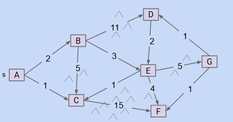
BFS does not always find the shortest path.

BFS simply gives us a path that contains the least intermediary nodes.
- If our graph was a weighted graph, then each edge could have different weights. The smallest number of nodes does not necessarily mean the smallest sum of weights.
To find the actual shortest path, we’ll need to create an algorithm that takes care of the weights in a graph as well.

There will never be a cycle in any shortest path between two nodes, a cycle means redundancy in our path.
Our problem to solve is that we want to find the shortest path from the source vertex s to every other vertex in our graph.
- My idea is that we can slowly keep track of the shortest path from s to its neighbors, and use that information to find the shorest distance from s to the neighbors of its neighbors, and so on.
- The shortest path from s to all its neighbors will mostly follow the same paths as the shortest path would rely on the shortest path from s to some neighbor of the vertex v that we want to reach.
  - Our shortest paths will have other shortest paths as its intermediates.
The solution will always be a tree if we have unique shortest paths.
- This is because the tree is just the union of the shortest paths of all vertices.
- By the definition of a graph, there will be $ V -1$ number of edges that connect all edges in the shortest paths tree of G. Assuming all vertices are reachable.

Start with all vertices unmarked, and all distances set to infinity. No edges in shortest path tree yet.
Start by marking the source node, and se sequentially remove a vertex from our friend and mark it.
For each outgoing edge, if the destination vertex is not a part of our SPT, we add the edge and add $w$ to our fringe.
This algorithm does not work.
- It considers vertices one “level” at a time, as the weights could be different values.

We create a new graph by adding many dummy nodes along an edge and then we run BFS. The dummy nodes represents the number of weights we have along the tree.
- Once we hit our original nodes, we add the edge to the SPT.
While this approach works, it consumes too much memory, as we are creating a lot of dummy nodes for no reason.
Also if we have weights that have a large number, then we have to traverse through many layers of dummy nodes until we hit our desired node.
Also, our implementation wouldn’t work for fractional weights.

Start by adding the source to the fringe.
While the fringe is not empty, remove the closest vertex from the fringe and mark it
For each outgoing edge v->w, if w is not already part of SPT, add the edge, and add w to fringe.
However, this approach is too greedy, as we are giving up potential paths in the future that are better.

We follow the Best-First Search idea but we consider our best path tentatively.
- We will go back in the future if we find a better, faster path to a previous node.
- We will use a priority queue to keep track of these distances.
Procedure:
- We add all vertices to the fringe.
- While the fringe is not empty:
  - We remove the closest vertex from the fringe and mark it.
  - For each outgoing edge v->w: if the edge gives a better distance to w, we add the edge and update w in the fringe.
Dijkstra can fail if a graph has negative edge weights.
Overall runtime: $O(V\cdot\log(V)+V\cdot\log(V)+E\cdot\log(V))$.

With only a sinle target, we can come up with a much faster heurustic method.
We will add a heuristic to dijkstras to ignore paths that will take us further away from our target.
The A* heuristic must satisfy two conditions:
- Admissible $h(b, NYC)\leq$